P1. (히스토그램 평활화) 다음 두개의 사진(Unequalized_Hawkes_Bay_NZ.jpg, tsukuba_l.png)에 히스토그램평활화를 적용하려고 한다.
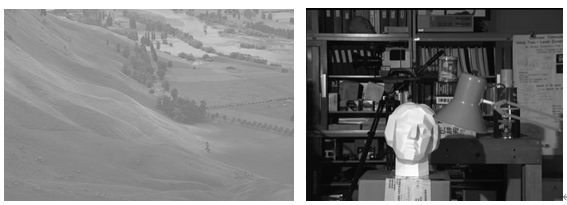
1) 위 사진의 히스토그램을 구하여 그래프로 표시해보라. (GRAY 영상으로 변환 후)
<코드>
| ''' 1. 위 사진의 히스토그램을 구하여 그래프로 표시해보라. (GRAY 영상으로 변환 후) ''' imgpath1='histo1.png' imgpath2='histo2.png' #color to gray histo1_gray = cv2.imread('histo1.png', cv2.IMREAD_GRAYSCALE) cv2.imwrite('histo1_gray.png', histo1_gray, [cv2.IMWRITE_PNG_COMPRESSION, 0]) histo1_gray = cv2.imread('histo1_gray.png', cv2.IMREAD_GRAYSCALE) histo2_gray = cv2.imread('histo2.png', cv2.IMREAD_GRAYSCALE) cv2.imwrite('histo2_gray.png', histo2_gray, [cv2.IMWRITE_PNG_COMPRESSION, 0]) histo2_gray = cv2.imread('histo2_gray.png', cv2.IMREAD_GRAYSCALE) #for test ''' plt.subplot(2,1,1) plt.imshow(histo1_gray) plt.subplot(2,1,2) plt.imshow(histo2_gray) ''' #find histogram hist1 = cv2.calcHist([histo1_gray], channels =[0], mask = None, histSize=[256],ranges=[0.0,256.0]) hist2 = cv2.calcHist([histo2_gray], channels =[0], mask = None, histSize=[256],ranges=[0.0,256.0]) #show histogram graph plt.plot(hist1) plt.title('hist1') plt.show() plt.plot(hist2) plt.title('hist2') plt.show() |
<결과>
Histogram of Unequalized_Hawkes_Bay_NZ.jpg
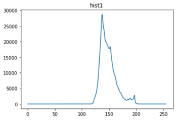
Histogram of tsukuba_l.png
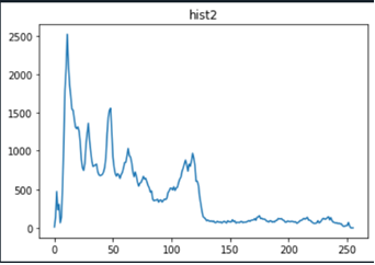
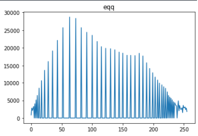
2) (전역) 히스토그램 평활화를 적용하고 그래프로 그려보라.
<코드>
| ''' 2. (전역) 히스토그램 평활화를 적용하고 그래프로 그려보라. ''' #1번 이미지 #평활화 함수. 리턴값은 평활화된 이미지임 histo1_gray_eq = cv2.equalizeHist(histo1_gray) #평활화된 이미지의 히스토그램 계산 hist1_eq = cv2.calcHist([histo1_gray_eq], channels =[0], mask = None, histSize=[256],ranges=[0.0,256.0]) plt.plot(hist1_eq) plt.title('equalization1') plt.show() plt.subplot(1,2,1) plt.imshow(histo1_gray_eq, cmap='gray') plt.title('equalization') plt.subplot(1,2,2) plt.imshow(histo1_gray, cmap='gray') plt.title('original') plt.show() #2번 이미지 #평활화 함수. 리턴값은 평활화된 이미지임 histo2_gray_eq = cv2.equalizeHist(histo2_gray) #평활화된 이미지의 히스토그램 계산 hist2_eq = cv2.calcHist([histo2_gray_eq], channels =[0], mask = None, histSize=[256],ranges=[0.0,256.0]) plt.plot(hist2_eq) plt.title('equalization2') plt.show() plt.subplot(1,2,1) plt.imshow(histo2_gray_eq, cmap='gray') plt.title('equalization') plt.subplot(1,2,2) plt.imshow(histo2_gray, cmap='gray') plt.title('original') plt.show() |
<결과>
Equalized Histogram of Unequalized_Hawkes_Bay_NZ.jpg
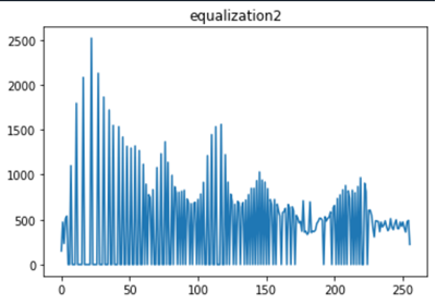
Equalized Histogram of tsukuba_l.png
3) 적응 히스토그램을 적용하여 보라 (OpenCV의 CLAHE: contrast limited adaptive histogram equalization를 사용하라.) 그리고 결과 영상의 히스토그램을 그려보라.
<코드>
| ''' 3. 적응 히스토그램을 적용하여 보라 (OpenCV의 CLAHE: contrast limited adaptive histogram equalization를 사용하라.) 그리고 결과 영상의 히스토그램을 그려보라 ''' #적응형히스토그램: 히스토그램을 이미지 전체가 아닌 tileGridSize 영역에 제한하여 따로 적용. #입력이미지의 히스토그램이 넓게 퍼져 있을때 사용하기 좋다. #1번 이미지 #CLAHE 커널 생성?? 리미트는 뭔소린지 모르겠고 두번쨰 패러미터는 각각의 영역 지정해주는 듯 clahe1=cv2.createCLAHE(clipLimit=2.0, tileGridSize=(8,8)) histo1_gray_CLAHE = clahe1.apply(histo1_gray) #히스토그램 계산 hist1_eq_CLAHE = cv2.calcHist([histo1_gray_CLAHE], channels =[0], mask = None, histSize=[256],ranges=[0.0,256.0]) #2번 이미지 clahe2=cv2.createCLAHE(clipLimit=2.0, tileGridSize=(8,8)) histo2_gray_CLAHE = clahe2.apply(histo2_gray) #히스토그램 계산 hist2_eq_CLAHE = cv2.calcHist([histo2_gray_CLAHE], channels =[0], mask = None, histSize=[256],ranges=[0.0,256.0]) #결과영상및 히스토그램 출력 plt.subplot(1,2,1) plt.imshow(histo1_gray_CLAHE, cmap='gray') plt.title('CLAHE img 1') plt.subplot(1,2,2) plt.imshow(histo2_gray_CLAHE, cmap='gray') plt.title('CLAHE img 2') plt.show() plt.subplot(1,2,1) plt.plot(hist1_eq_CLAHE) plt.title('CLAHE histogram 1') plt.subplot(1,2,2) plt.plot(hist2_eq_CLAHE) plt.title('CLAHE histogram 2') plt.show() |
<결과>
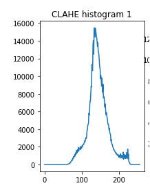
CLAHE Equalized Histogram of Unequalized_Hawkes_Bay_NZ.jpg
CLAHE Equalized Histogram of tsukuba_l.png
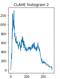
4) 2와 3의 결과를 비교하고 그 차이의 원인이 무엇인지 설명하라.
2번의 경우 영상 전체에 대해 히스토그램 평활화를 적용하였으나 3번의 경우 이미지를 작은 부분공간으로 나누어 (작성한 코드에서는 8by8 이미지) 각각 평활화를 적용하기 때문에 히스토그램 그래프 또한 부분적으로 평활화되어있음을 확인할수 있다.
P2. (히스토그램 역투영) 모델의 색분포를 이용한 얼굴 검출을 해본다.
1) 우선 모델 히스토그램은 다음 이미지를 사용하자.
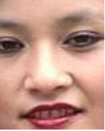
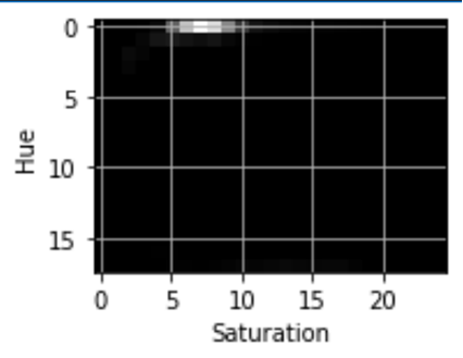
위 이미지를 HSV 색상으로 변환하고 이중 H와 S를 사용한 2차원 히스토그램을 구하고 이를 보여라.
<코드>
| ''' 1. 우선 모델 히스토그램은 다음 이미지를 사용하자. 위 이미지를 HSV 색상으로 변환하고 이중 H와 S를 사용한 2차원 히스토그램을 구하고 이를 보여라. ''' import numpy as np import matplotlib.pyplot as plt import cv2 modelhis = cv2.imread('face.png') modelhis = cv2.cvtColor(modelhis, cv2.COLOR_BGR2HSV) #channel을 [0,1]만 사용 즉 HSV에서 HS만 사용하여 모델의 히스토그램 계산 hist_model = cv2.calcHist([modelhis], channels =[0,1], mask = None, histSize=[18, 25],ranges=[0.,181., 0., 256.]) plt.subplot(1,2,1) plt.imshow(hist_model, cmap='gray') plt.xlabel('Saturation') plt.ylabel('Hue') plt.grid() plt.show() |
<결과>
히스토그램:
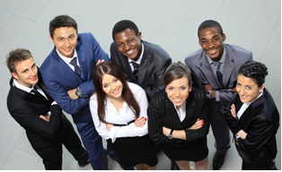
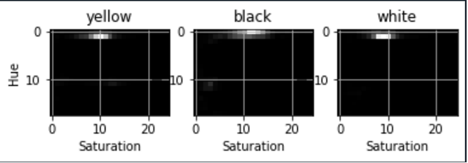
2) 다음 이미지의 전체 영역의 HS 히스토그램을 구해 보고, 황인(윗줄 맨왼쪽 남자), 흑인(윗줄 오른쪽), 백인 (아랫줄 우측 두번째 여성)의 얼굴 부분을 선택하여 HS 히스토그램을 구하고 비교해보라
<코드>
| ''' 2. 다음 이미지의 전체 영역의 HS 히스토그램을 구해 보고, 황인(윗줄 맨왼쪽 남자), 흑인(윗줄 오른쪽), 백인 (아랫줄 우측 두번째 여성)의 얼굴 부분을 선택하여 HS 히스토그램을 구하고 비교해보라 ''' #각각 얼굴파일 불러오고 HSV로 변환 yellow = cv2.imread('yellow.png') yellow = cv2.cvtColor(yellow, cv2.COLOR_BGR2HSV) black = cv2.imread('black.png') black = cv2.cvtColor(black, cv2.COLOR_BGR2HSV) white = cv2.imread('white.png') white = cv2.cvtColor(white, cv2.COLOR_BGR2HSV) #H,S에 대해 히스토그램 계산 his_yellow = cv2.calcHist([yellow], channels =[0,1], mask = None, histSize=[18, 25],ranges=[0.,181., 0., 256.]) his_black = cv2.calcHist([black], channels =[0,1], mask = None, histSize=[18, 25],ranges=[0.,181., 0., 256.]) his_white = cv2.calcHist([white], channels =[0,1], mask = None, histSize=[18, 25],ranges=[0.,181., 0., 256.]) #히스토그램 출력 plt.subplot(1,3,1) plt.imshow(his_yellow, cmap='gray') plt.title('yellow') plt.xlabel('Saturation') plt.ylabel('Hue') plt.grid() plt.subplot(1,3,2) plt.imshow(his_black, cmap='gray') plt.title('black') plt.xlabel('Saturation') plt.ylabel('Hue') plt.grid() plt.subplot(1,3,3) plt.imshow(his_white, cmap='gray') plt.title('white') plt.xlabel('Saturation') plt.ylabel('Hue') plt.grid() plt.show() #HS영역 보기(확인용) HS_total=((his_black)+(his_white)+(his_yellow))/3 print(HS_total) plt.imshow(HS_total, cmap='gray') plt.title('total') plt.show() |
<결과>
황인, 흑인, 백인 얼굴에 대한 히스토그램은 아래와 같다:
3) 앞서 결과를 바탕으로 눈 대중으로 얼굴에 해당하는 HS 영역을 정의해 보라.
위의 결과로부터 얼굴에 해당하는 HS 영역은 H: 5~20, S: 50~150 영역이다.
4) 위의 이미지를 사용하여 히스토그램 역투영방식을 사용하여 얼굴 영역을 검출하고 위의 결과와 비교 해보라.
<코드>
| ''' 4. 위의 이미지를 사용하여 히스토그램 역투영방식을 사용하여 얼굴 영역을 검출하고 위의 결과와 비교 해보라. ''' def facefinder(img): #입력이미지 크기 계산 ysize, xsize, th = img.shape backpro=np.zeros((ysize,xsize)) for y in range(img.shape[0]): for x in range(img.shape[1]): h,s,v = img[y][x] if(5<=h & h<=20 & 50<=s & s<=150): backpro[y][x] = 1 return backpro people=cv2.imread('people.png') people=cv2.cvtColor(people, cv2.COLOR_BGR2HSV) ans=facefinder(people) plt.imshow(ans, cmap='gray') plt.title('face area') plt.show() |
<결과>
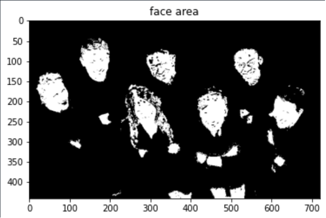
사진속의 모든 얼굴이 성공적으로 검출되었으나 얼굴과 비슷한 색상을 가지는 손, 가슴, 다리 등 또한 함께 검출되었다.
P4. 이전 문제에서 얻은 역투영 상식의 사용한 얼굴화소검출 에 대한 결과를 이용하여 얼굴 영역 검출을 하려고 한다.
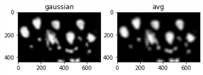
1) 우선 위에서 구한 이미지를 평균/가우시안 필터를 사용하여 스무딩을 적용하라.
<코드>
| people=cv2.imread('backpro.png') people=cv2.cvtColor(people, cv2.COLOR_BGR2RGB) #가우시안 스무딩 gauss=cv2.GaussianBlur(people,(31,31),10) #평균 스무딩 #커널생성 k_size=31 kernel = np.ones((k_size,k_size),np.float32)/(k_size*k_size) #스무딩 적용 avg = cv2.filter2D(people,-1,kernel) plt.subplot(1,2,1) plt.imshow(gauss) plt.title('gaussian') plt.subplot(1,2,2) plt.imshow(avg) plt.title('avg') plt.show() |
<결과>
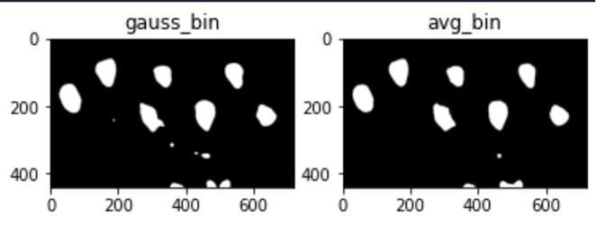
2) Otsu 알고리즘을 사용하여 임계치 T를 정하고, 반영하여 이진화를 수행하라. 또는 Otsu에서 구해진 임계치를 바탕으로 수정하라.
<코드>
| cv2.imwrite('gauss_gray.png', gauss, [cv2.IMWRITE_PNG_COMPRESSION, 0]) gauss_gray=cv2.imread('gauss_gray.png', cv2.IMREAD_GRAYSCALE) cv2.imwrite('avg_gray.png', avg, [cv2.IMWRITE_PNG_COMPRESSION, 0]) avg_gray=cv2.imread('avg_gray.png', cv2.IMREAD_GRAYSCALE) thres_g, gauss_bin = cv2.threshold(gauss_gray, thresh = 0 , maxval = 255, type = cv2.THRESH_BINARY + cv2.THRESH_OTSU) print('gauus thres') print(thres_g) thres_a, avg_bin = cv2.threshold(avg_gray, thresh = 0 , maxval = 255, type = cv2.THRESH_BINARY + cv2.THRESH_OTSU) print('avg thres') print(thres_a) thres_g2, gauss_bin2 = cv2.threshold(gauss_gray, thresh = thres_g +80, maxval = 255, type = cv2.THRESH_BINARY) thres_a2, avg_bin2 = cv2.threshold(avg_gray, thresh = thres_a +80, maxval = 255, type = cv2.THRESH_BINARY) #이진화영상 plt.subplot(1,2,1) plt.imshow(gauss_bin2, cmap='gray') plt.title('gauss_bin') plt.subplot(1,2,2) plt.imshow(avg_bin2, cmap='gray') plt.title('avg_bin') plt.show() |
<결과>
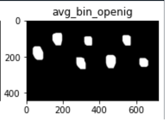
3) 형태학적 필터 (erode, dilate, open 또는 close 등)을 적절히 사용하여 얼굴 영역을 검출해보라.
<코드>
| #미세한 점들이 많으므로 Opening: Dilation after erosion 적용 #avg filter의 결과값이 더 적합하므로 avg 결과영상에만 적용 #커널생성 kernel = np.ones((10,10),np.uint8) #비교용 이미지 #Opening ite=3 avg_bin_erode = cv2.erode(avg_bin2,kernel,iterations = ite) avg_bin_open = cv2.dilate(avg_bin_erode,kernel,iterations = ite) plt.subplot(1,2,1) plt.imshow(avg_bin2, cmap='gray') plt.title('avg_bin_original') plt.subplot(1,2,2) plt.imshow(avg_bin_open, cmap='gray') plt.title('avg_bin_openig') plt.show() |
<결과>
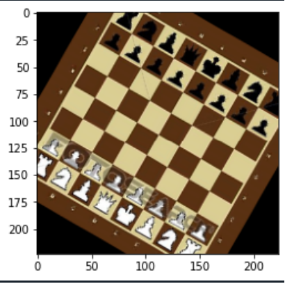
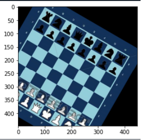
P4. (기하변환) 다음 체스판 이미지를 사용하여 실습을 수행하라.
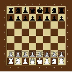
1) 체스 판을 1/2로 축소하고, 이미지 중심에서 30도 시계방향으로 회전 해보라. (getRotationMatrix2D를 활용). 이 때 생성된 Matrix 를 프린트하고 이를 설명하라.
<코드>
| import numpy as np import cv2 import matplotlib.pyplot as plt ''' [문제가 모호하여 채점에 참고 하겟음.] (기하변환) 다음 체스판 이미지를 사용하여 실습을 수행하라. ''' ''' 1) 체스 판을 1/2로 축소하고, 이미지 중심에서 30도 시계방향으로 회전 해보라. (getRotationMatrix2D를 활용). 이 때 생성된 Matrix 를 프린트하고 이를 설명하라. ''' chess_orig = cv2.imread('chess.png') chess_orig = cv2.cvtColor(chess_orig, cv2.COLOR_BGR2RGB) xsize=chess_orig.shape[0] ysize=chess_orig.shape[1] #새로운 사이즈(1/2) #정수값이 필요하므로 // 연산자 사용 resize = (xsize//2, ysize//2) chess_half = cv2.resize(chess_orig, resize, interpolation = cv2.INTER_NEAREST) #축소된 사이즈 체크용 print('original size = ', xsize, ysize) print('after = ', resize) xsize_r, ysize_r = resize #시게방향 30도 회전 #회전행렬생성 #중심점, 각도, 스케일. 이때 //이 버림연산이므로 +1을 하면 정확한 중앙좌표 RM = cv2.getRotationMatrix2D( (xsize_r//2 + 1 , ysize_r//2 + 1), -30, 1.0) #Affine transform에 RM 커널 적용 chess_rotate = cv2.warpAffine(chess_half, RM, (xsize_r, ysize_r)) plt.imshow(chess_rotate) plt.show() print('rotation matrix = ', RM) |
<결과>
회전 및 축소 결과:
행렬 출력:

생성된 회전행렬의 경우 2행 3열의 행렬인데, 처음 2행 2열의 성분들은 기존에 알고있던 2차원 회전행렬
에 각도 -30 degree 를 적용한 값과 동일하고, 3열 성분은 회전 중심점, 회전시 스케일에 관련된 양으로 생각된다.
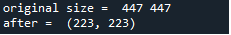
또한 이미지 사이즈 또한 1/2로 성공적으로 줄어들었음을 확인하였다.
2) 앞서 결과를 이용하여 체스 판을 1/2로 축소하고, 이미지 중심에서 30도 시계방향으로 회전 후 (30, 20)만큼 이동하여 보라.
<코드>
| import numpy as np import cv2 import matplotlib.pyplot as plt ''' [문제가 모호하여 채점에 참고 하겟음.] (기하변환) 다음 체스판 이미지를 사용하여 실습을 수행하라. ''' ''' 1) 체스 판을 1/2로 축소하고, 이미지 중심에서 30도 시계방향으로 회전 해보라. (getRotationMatrix2D를 활용). 이 때 생성된 Matrix 를 프린트하고 이를 설명하라. ''' chess_orig = cv2.imread('chess.png') chess_orig = cv2.cvtColor(chess_orig, cv2.COLOR_BGR2RGB) xsize=chess_orig.shape[0] ysize=chess_orig.shape[1] #새로운 사이즈(1/2) #정수값이 필요하므로 // 연산자 사용 resize = (xsize//2, ysize//2) chess_half = cv2.resize(chess_orig, resize, interpolation = cv2.INTER_NEAREST) #축소된 사이즈 체크용 print('original size = ', xsize, ysize) print('after = ', resize) xsize_r, ysize_r = resize #시게방향 30도 회전 #회전행렬생성 #중심점, 각도, 스케일. 이때 //이 버림연산이므로 +1을 하면 정확한 중앙좌표 #좌표이동을 위해 회전중심점 이동 RM = cv2.getRotationMatrix2D( (xsize_r//2 + 31 , ysize_r//2 + 21), -30, 1.0) #Affine transform에 RM 커널 적용 chess_rotate = cv2.warpAffine(chess_half, RM, (xsize_r, ysize_r)) plt.imshow(chess_rotate) plt.show() print('rotation matrix = ', RM) |
<결과>
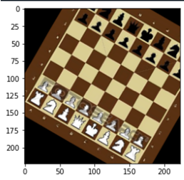
3) 위에서 Affine Warping을 하기 점-매칭을 이용하여 Matrix를 구해보고 이를 분석하여 보라.
<코드>
Afiine Warping을 위한 3개의 좌표쌍을 얻기 위해 회전행렬을 구하고 임의의 점 3개를 선택하여 결과점을 계산한다. 계산은 Matlab을 사용하였고,
이에 대한 코드는 다음과 같다:
| ''' 3) 위에서 Affine Warping을 하기 점-매칭을 이용하여 Matrix를 구해보고 이를 분석하여 보라. ''' chess_orig_affine = cv2.imread('chess.png') chess_orig_affine = cv2.cvtColor(chess_orig, cv2.COLOR_BGR2RGB) xsize=chess_orig_affine.shape[0] ysize=chess_orig_affine.shape[1] #이 3개 점 좌표를 points1 = np.float32([[300,300],[320,320],[340,340]]) #각각 여기로 이동 points2 = np.float32([[105,28],[132,35],[159,42]]) #Affine matrix 생성 RM_affine = cv2.getAffineTransform(points1, points2) #affine transform된 이미지 afteraffine = cv2.warpAffine(chess_orig_affine, RM, (xsize, ysize)) print('','Rotationmatrix = ', RM_affine) plt.imshow(chess_orig_affine) plt.show() plt.imshow(afteraffine) plt.show() |
<결과>
P5. (기하변환) 다음 수업에서 연습으로 사용한 그림에 대하여 다음 실험을 해보자.
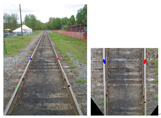
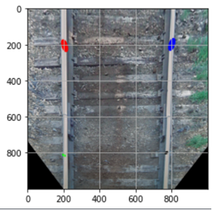
1) 원영상과 변환된 영상에서 대응되는 4개를 마킹점의 좌표 값을 읽고, 그 좌표쌍을 이용하여 PerspectiveWarping 을 해보시오.
<코드>
| import numpy as np import cv2 import matplotlib.pyplot as plt ''' P5. (기하변환) 다음 수업에서 연습으로 사용한 그림에 대하여 다음 실험을 해보자 ''' ''' 1) 원영상과 변환된 영상에서 대응되는 4개를 마킹점의 좌표 값을 읽고, 그 좌표쌍을 이용하여 PerspectiveWarping 을 해보시오. ''' train = cv2.imread('train.png') train_bird = cv2.imread('train_bird.png') #점의 좌표값을 알아내기 위해 grid 함수를 사용한다. plt.imshow(train) plt.grid() plt.show() plt.imshow(train_bird) plt.grid() plt.show() # 좌표의 이동전의 점: 좌상->좌하->우상->우하 pts1 = np.float32([[500,1000],[250,1500], [1000,1000],[1250,1500] ]) # 좌표의 이동후의 점 pts2 = np.float32([[200,200],[200,800], [800,200],[800,800]]) PM = cv2.getPerspectiveTransform(pts1, pts2) # matrix 계산 train_bird = cv2.warpPerspective(train, PM, (1000,1000)) plt.imshow(train_bird) plt.title('after transform') plt.show() |
<결과>
2) 동일한 작업을 Affine 변환을 사용하여 (임을 3점을 선택하여 사용) 해보라
<코드>
| ''' 2) 동일한 작업을 Affine 변환을 사용하여 (임을 3점을 선택하여 사용) 해보라. ''' #이 3개 점 좌표를 points1 = np.float32([[500,1000],[250,1500],[1000,1000]]) #각각 여기로 이동 points2 = np.float32([[200,200],[200,800],[800,200]]) #Affine matrix 생성 Per_affine = cv2.getAffineTransform(points1, points2) #affine transform된 이미지 train_affine = cv2.warpAffine(train, Per_affine, (1000, 1000)) plt.imshow(train_affine) plt.show() |
<결과>
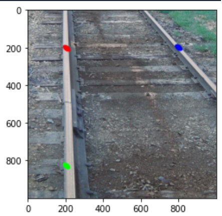
3) 위 두 결과를 비교 해보라.
좌표쌍 4개를 사용하는 Perspective transform과 달리 좌표쌍 3개만 사용한 Affine transform의 결과가 각각 다름을 확인할수 있다.
특히 Affine transform에서 붉은색 점과 초록색 점이 위치한 선로는 나름 수직선으로 성공적으로 변환되었으나 오른쪽의 선로는 좌표쌍이 부족하여 (perspective transform같은)시점변환이 아닌 단순 매핑으로 이루어져 두 변환이 동일한 결과를 가져오지 못하였다.
P6. (컬러 이미지 이퀄라이제이션) 컬러 영상의 이퀄라이제이션은 어떻게 하는 것이 좋을까?
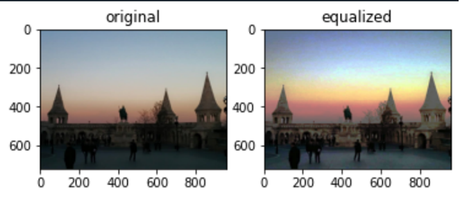
1) 첫번째 생각할 수 있는 방법은 각 채널 당하는 것이다. RGB 각 채널에대하여 histogram equalization을 적용한 후 다시 합치는 방식으로 영상을 처리해보고 결과를 확인하라.
<코드>
| import numpy as np import cv2 import matplotlib.pyplot as plt ''' P6. (컬러 이미지 이퀄라이제이션) 컬러 영상의 이퀄라이제이션은 어떻게 하는 것이 좋을까? ''' ''' 1) 첫번째 생각할 수 있는 방법은 각 채널 당하는 것이다. RGB 각 채널에대하여 histogram equalization을 적용한 후 다시 합치는 방식으로 영상을 처리해보고 결과를 확인하라. ''' img=cv2.imread('problem6.png') img=cv2.cvtColor(img, cv2.COLOR_BGR2RGB) #cv2.split 함수: 각 채널별로 쪼개기 img_R, img_G, img_B = cv2.split(img) #각 채널에 대해 히스토그램 찾기 his_R = cv2.calcHist(img, channels = [0], mask = None, histSize = [256], ranges=[0.0,256.0]) his_G = cv2.calcHist(img, channels = [1], mask = None, histSize = [256], ranges=[0.0,256.0]) his_B = cv2.calcHist(img, channels = [2], mask = None, histSize = [256], ranges=[0.0,256.0]) img_R_eq = cv2.equalizeHist(img_R,his_R) img_G_eq = cv2.equalizeHist(img_G,his_G) img_B_eq = cv2.equalizeHist(img_B,his_B) #cv2.merge 함수: 이미지 다시 합치기 img_eq=cv2.merge((img_R_eq, img_G_eq, img_B_eq)) plt.subplot(1,2,1) plt.imshow(img) plt.title('original') plt.subplot(1,2,2) plt.imshow(img_eq) plt.title('equalized') |
<결과>
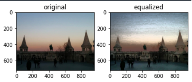
2) 또다른 방법은 RGB 채널을 HSV로 변환한 후 V 채널에만 Histogram Equalization을 적용하고 그 결과를 확인해보라.
<코드>
| ''' 2) 또다른 방법은 RGB 채널을 HSV로 변환한 후 V 채널에만 Histogram Equalization을 적용하고 그 결과를 확인해보라. ''' img=cv2.cvtColor(img, cv2.COLOR_RGB2HSV) #cv2.split 함수: 각 채널별로 쪼개기 img_H, img_S, img_V = cv2.split(img) #V 채널에 대해 히스토그램 찾기 his = cv2.calcHist(img, channels = [2], mask = None, histSize = [256], ranges=[0.0,256.0]) img_V_eq = cv2.equalizeHist(img_V,his) print('test = ', img_V - img_V_eq) #cv2.merge 함수: 이미지 다시 합치기 img_eq=cv2.merge((img_H, img_S, img_V_eq)) img_eq=cv2.cvtColor(img_eq, cv2.COLOR_HSV2RGB) img=cv2.cvtColor(img, cv2.COLOR_HSV2RGB) plt.subplot(1,2,1) plt.imshow(img) plt.title('original') plt.subplot(1,2,2) plt.imshow(img_eq) plt.title('equalized') |
<결과>
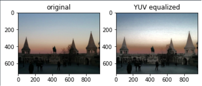
3) 또다른 방식으로 수업에서는 안 배웠지만, YUV 컬러스페이스라는 것이 있다. 사용법은 HSV와 비슷한데 Y는 Luminance를 의미하고 나머지는 Blue와 Red에 대한 대략적인 색상 정보를 의미한다. 앞서와 마찬가지로 YUV에서 Y에 대하여 Histogram Equalizer를 적용하고 결과를 보자.
<코드>
| ''' 3) 또다른 방식으로 수업에서는 안 배웠지만, YUV 컬러스페이스라는 것이 있다. 사용법은 HSV와 비슷한데 Y는 Luminance를 의미하고 나머지는 Blue와 Red에 대한 대략적인 색상 정보를 의미한다. 앞서와 마찬가지로 YUV에서 Y에 대하여 Histogram Equalizer를 적용하고 결과를 보자. ''' img=cv2.cvtColor(img, cv2.COLOR_RGB2YUV) #cv2.split 함수: 각 채널별로 쪼개기 img_Y, img_U, img_V = cv2.split(img) #Y 채널에 대해 히스토그램 찾기 his = cv2.calcHist(img, channels = [0], mask = None, histSize = [256], ranges=[0.0,256.0]) img_Y_eq = cv2.equalizeHist(img_Y,his) print('test = ', img_Y - img_Y_eq) #cv2.merge 함수: 이미지 다시 합치기 img_eq_YUV=cv2.merge((img_Y_eq, img_U, img_V)) img_eq_YUV=cv2.cvtColor(img_eq_YUV, cv2.COLOR_YUV2RGB) img=cv2.cvtColor(img, cv2.COLOR_YUV2RGB) plt.subplot(1,2,1) plt.imshow(img) plt.title('original') plt.subplot(1,2,2) plt.imshow(img_eq_YUV) plt.title('YUV equalized') |
<결과>
4) 이 3개의 결과 차이에 대하여 논의해보라.
먼저 RGB 이퀄라이제이션의 경우, 밝기값이 아닌 색상에 대해서만 이퀄라이제이션을 적용하였기 때문에 HSV나 YUV 에 비해 색상왜곡이 많이 발생하였다. (하늘 색상이 왜곡)
참고 자료
컴퓨터 비전(Computer Vision)
기본 개념부터 최신 모바일 응용 예까지-
저자오일석
-
출판한빛아카데미
-
출간2014.07.30.
'프로그래밍 > 영상처리공학' 카테고리의 다른 글
| [영상처리공학/OpenCV with python]연주 영상 인식 피아노 (0) | 2022.12.19 |
|---|---|
| [HW 3]에지 검출과 영역 분할 (0) | 2022.12.19 |
| [HW 1]영상처리 기본, Python & OpenCV (0) | 2022.12.18 |