[HW 3]에지 검출과 영역 분할

프로그래밍/영상처리공학

[HW 3]에지 검출과 영역 분할

RAVIN 2022. 12. 19. 16:11

P1. (SOBEL 에지) 다음과 같은 Grayscale 이미지를 만들어 각각 실험하라.

1) 위와 유사하게 원과 정사각형 도형이 그려진 이미지를 만들어라.

<코드>

import cv2
import numpy as np
import matplotlib.pyplot as plt

'''
1) 위와 유사하게 원과 정사각형 도형이 그려진 이미지는 만들어라.
'''

#이미지 그릴 배경 그리기
im_circle = np.zeros([500, 500, 3], dtype= np.uint8)
im_rect = np.zeros([500, 500, 3], dtype= np.uint8)

center = (250, 250)

#draw circle
#패러미터: 반지름, 색상, 두께 -1(채워진 도형)
im_circle = cv2.circle(im_circle, center, 100, color =(255,255,255), thickness=-1)

#draw rectangle

#각 대각선 좌표지정
pt1 = (150, 150)
pt2 = (350, 350)
#패러미터: 대상이미지, 대각좌표, 색상, 두께 -1
im_rect = cv2.rectangle(im_rect, pt1, pt2, color = (255,255,255), thickness=-1)

plt.subplot(1,2,1)
plt.imshow(im_circle)
plt.title('circle')

plt.subplot(1,2,2)
plt.imshow(im_rect)
plt.title('rectangle')

plt.show()

<결과>

2) Sobel 에지를 수평, 수직 측으로 구하고 (kernel size = 3), 여기서 magnitude 이미지를 이진화 하라. (오츄 알고리즘 등 사용)

<코드 - SOBEL 에지>

<결과 - SOBEL 에지>

<코드 - magnitude 이진화>

def mySobel(src,c):
    #소벨 이미지 생성
    gx = cv2.Sobel(src, cv2.CV_32F, 1, 0, ksize = 3) # x order = 1 only
    gy = cv2.Sobel(src, cv2.CV_32F, 0, 1, ksize = 3) # y

    if(c==1):
        #sobel 이미지 출력하기
        plt.subplot(1,2,1)
        plt.imshow(gx,cmap='gray')
        plt.title('horizintal sobel')

        plt.subplot(1,2,2)
        plt.imshow(gy,cmap='gray')
        plt.title('vertical sobel')

        plt.show()
    else:
        #magnitude 이미지 리턴

        #카테시안에서 극좌표로 바꾸기. 다만 angle값이 0~360 까지 나온다.
        #에지의 각도는 0~180까지이기 때문에 이래 해줘야 함. ㅇㅇ
        mag, angle = cv2.cartToPolar(gx, gy, angleInDegrees=True)
        dstM   = cv2.magnitude(gx, gy)
        minVal, maxVal, minLoc, maxLoc = cv2.minMaxLoc(dstM)

        #이미지파일(3차원)으로 변환하는 코드
        dstM = cv2.normalize(dstM, None, 0, 255, cv2.NORM_MINMAX, dtype=cv2.CV_8U)
        return dstM

#magnitude 이미지 생성
mag_circle = mySobel(im_circle,0)
mag_rect = mySobel(im_rect,0)

plt.subplot(1,2,1)
plt.imshow(mag_circle, cmap='gray')

plt.subplot(1,2,2)
plt.imshow(mag_rect, cmap='gray')

def mybin(src):
    #이진화
    thres, im_bin = cv2.threshold(src, thresh = 0 , maxval = 255, type = cv2.THRESH_BINARY + cv2.THRESH_OTSU)

    plt.imshow(im_bin,cmap='gray')
    plt.show()

    return im_bin

mag_circle_bin = mybin(mag_circle)
mag_rect_bin = mybin(mag_rect)

plt.subplot(1,2,1)
plt.imshow(mag_circle_bin, cmap='gray')
plt.title('bin')

plt.subplot(1,2,2)
plt.imshow(mag_rect_bin, cmap='gray')
plt.title('bin')

plt.show()

<결과 - magnitude 이진화>

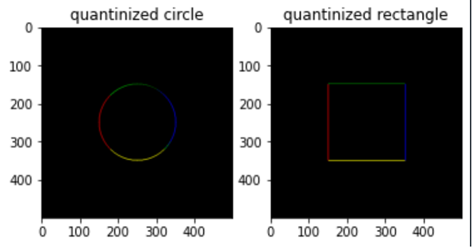
3) 이진화된 에지영역에서 gradient을 구하고 이를 4개의 영역으로 양자화 하고 각 영역 별로 다음과 같이 색을 매칭하여 이미지를 만들어라. (즉, -45 - 45 도: 빨강, 45 – 135.5: 녹색, 135 - 225: 파랑, 225- -45도: 노랑).

<코드>

def quatiangle(src):
    #각도 찾기를 위한 그래디언트 구하기
    gx = cv2.Sobel(src, cv2.CV_32F, 1, 0, ksize = 3)
    gy = cv2.Sobel(src, cv2.CV_32F, 0, 1, ksize = 3)


    #앵글계산
    angles = np.arctan(gy/gx)
    print("nan?", np.isnan(angles)) # some are NAN becuase deivide-by-zero

    #nan값을 0으로 바꾸는 함수. 반드시 필요!
    np.nan_to_num(angles, copy= False, nan=0.0) # replace by zero
    print("nan?", np.isnan(angles)) # some are NAN becuase deivide-by-zero
    print(cv2.minMaxLoc(angles))

    #radian -> degree 변환
    angles = angles/np.pi*180.0

    #이때 arctan 함수의 특성으로 인해 그래디언트 방향이 [-pi/2, pi/2]만 검출되는 문제 발생
    #다음 문제 진행을 위해 어쩔수 없이 x-y 평면상에서 그래프를 찾고 부등식을 사용하여 해결

    m=0
    n=0

    indexmat = np.zeros((500,500))

    print('initial', indexmat)
    while(m<500):
        while(n<500):
            if(m>n):
                indexmat[m][n] = 1
            n=n+1

        m=m+1
        n=0


    print('indexmat_2',indexmat)
    print('nonzero',np.count_nonzero(indexmat))

    angles[(indexmat == 1)] = angles[(indexmat == 1)] + 180


    m=0
    n=0

    indexmat = np.zeros((500,500))

    print('initial', indexmat)
    while(m<500):
        while(n<500):
            if((m>n) & (m>-n+500)):
                indexmat[m][n] = 1
            n=n+1

        m=m+1
        n=0


    print('indexmat_2',indexmat)
    print('nonzero',np.count_nonzero(indexmat))

    angles[(indexmat == 1)] = angles[(indexmat == 1)] + 180



    #각도의 양자화
    #양자화를 위한 인덱스 매트릭스 생성
    dstAngles = np.zeros([angles.shape[0], angles.shape[1]], dtype = np.uint8)

    #-45 ~ 45, R
    dstAngles[ (angles >= -45) & (angles < 45) ] = 1
    #45 ~ 135, G
    dstAngles[ (angles >= 45) & (angles < 135) ] = 2
    #135 ~ 225, B
    dstAngles[ (angles >= 135) & (angles < 255) ] = 3
    #255~-45, Y
    dstAngles[ angles >= 255 ] = 4

    dstAngles[src < 30] = 0 #0은 엣지가 아닌 부분 의미

    #angle test
    print('angle quantinization test:')
    print(np.count_nonzero(dstAngles[dstAngles == 1]))
    print(np.count_nonzero(dstAngles[dstAngles == 2]))
    print(np.count_nonzero(dstAngles[dstAngles == 3]))
    print(np.count_nonzero(dstAngles[dstAngles == 4]))
    print(np.count_nonzero(dstAngles[dstAngles == 0]))


    #출력용 컬러영상 배경 그리기
    im_black = np.zeros([500, 500, 3], dtype= np.uint8)

    im_black[dstAngles==1]=(0,0,255)
    im_black[dstAngles==2]=(0,255,0)
    im_black[dstAngles==3]=(255,0,0)
    im_black[dstAngles==4]=(255,255,0)

    plt.imshow(im_black)
    plt.title('final')
    plt.show()

    return im_black

#for test
quanti_circle = quatiangle(mag_circle_bin)
quanti_rect = quatiangle(mag_rect_bin)

plt.subplot(1,2,1)
plt.imshow(quanti_circle)
plt.title('quantinized circle')

plt.subplot(1,2,2)
plt.imshow(quanti_rect)
plt.title('quantinized rectangle')

<결과>

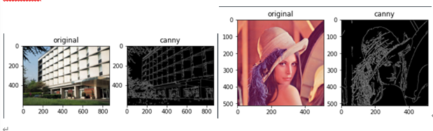
P2. (Canny 에지) 다음 두 이미지를 이용하여 캐니 에지 실험을 해본다.

1) T_high = 2.5 *T_low로 하면서 Tlow를 조절하여 파라메터를 사용하여 Canny 검출을 한 결과를 관찰하고 각각 영상에 가장 적절한 Tlow 값을 결정해보라.

<코드>

import cv2
import numpy as np
import matplotlib.pyplot as plt

'''
1) T_high = 2.5 *T_low로 하면서 Tlow를 조절하여 파라메터를 사용하여
Canny 검출을 한 결과를 관찰하고 각각 영상에 가장 적절한 Tlow 값을 결정해보라
'''

def mycanny(src,tl,var):
    orig = src
    th = 2.5*tl

    #가우시안 필터 적용
    if(var != -1):
        src = cv2.GaussianBlur(src, (0,0), var)
        th=tl

    #흑백영상으로 변환
    src_gray = cv2.cvtColor(src, cv2.COLOR_BGR2GRAY)

    #캐니에지 적용
    canny_src = cv2.Canny(src_gray, threshold1= th, threshold2 = tl)

    orig = cv2.cvtColor(orig, cv2.COLOR_BGR2RGB)
    plt.subplot(1,2,1)
    plt.imshow(orig)
    plt.title('original')

    plt.subplot(1,2,2)
    plt.imshow(canny_src,cmap='gray')
    plt.title('canny')

    plt.show()

img1 = cv2.imread('p2_1.png')
img2 = cv2.imread('p2_2.png')

mycanny(img1, 71, -1)

<결과>

위의 결과로부터 각각 순서대로 Tlow=71,55 로 설정하였을 때 결과가 가장 좋게 나오는 것을 확인하였다.

2) 위의 가우시안 필터 중에서 가장 맘에 드는 것을 하나를 정하고, T_high 와 T_low 를 같은 값으로 세팅하여 결과를 살펴 보라.

<코드>

'''
2)위의 가우시안 필터 중에서 가장 맘에 드는 것을 하나를 정하고,
T_high 와 T_low 를 같은 값으로 세팅하여 결과를 살펴 보라.
'''

mycanny(img1, 71, 1)
mycanny(img2, 55, 1)

<결과>

3) 1)의 실험을 Histogram Equalizer를 수행한 이후에 반복해보라.

<코드>

img1_hist = cv2.equalizeHist(img1)
img2_hist = cv2.equalizeHist(img2)

mycanny(img1_hist, 71, -1)
mycanny(img2_hist, 55, -1)

mycanny(img1_hist, 71, 1)
mycanny(img2_hist, 55, 1)

<결과 - 가우시안 필터 미적용>

<결과 - 가우시안 필터 적용>

P3. (Laplacian 필터) 다음 그림을 이용하여 구현 및 실험을 하시오.

1) 책의 (3.12) 식을 이용하여 LoG 필터의 커널을 만들어라. 그 결과를 책 그림 3-13과 비교 하라. (sigma = 0.5, 1.0, 2.0, 5.0).

<코드>

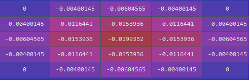
import cv2
import numpy as np
from matplotlib import pyplot as plt

'''
1)               책의 (3.12) 식을 이용하여 LoG 필터의 커널을 만들어라.
그 결과를 책 그림 3-13과 비교 하라. (sigma = 0.5, 1.0, 2.0, 5.0).
'''
def LOGkernel(ksize,sigma):
    #가우시안 커널 먼저 생성
    vector = cv2.getGaussianKernel(ksize, sigma)
    gkernel = np.outer(vector, vector.transpose())
    print('test:', gkernel)

    #LOG 커널 생성하기
    m,n = 0, 0
    center = ksize//2
    LOGker = np.zeros((ksize,ksize))

    while(m<ksize):
        while(n<ksize):
            #교재의 3.12 식은 커널의 원점이 (0,0)이라는 가정하에 유도된 식이기 때문에 적절한 좌표이동 적용.
            LOGker[m][n] = (((m-center)**2 + (n-center)**2 - 2*sigma**2)/(sigma**4)) * gkernel[m][n]
            n=n+1
        m=m+1
        n=0


   return LOGker

img=cv2.imread('p2_2.png')
Lkernel_0 = LOGkernel(3, 0.5)
Lkernel_1 = LOGkernel(7, 1)
Lkernel_2 = LOGkernel(13, 2)
Lkernel_5 = LOGkernel(31, 5)

<결과 - 시그마 0.5>

<결과 - 시그마 1>

<결과 - 시그마 2>

<결과 - 시그마 5>

2) 그림의 이미지를 이용하여 Gaussian Filter를 하고, Laplacian Filter를 차례대로 처리한 결과와 LOG 필터를 직접 적용한 결과를 차 영상을 만들어 비교하라 (sigma = 0.5, 1.0, 2.0, 5.0).

<코드>

def LOGcom(src,sigma,kernel):
    ksize = np.shape(kernel)
    print('test:',ksize)

    #Laplacian filtering after Gaussian filtering
    img1 = cv2.GaussianBlur(src,ksize,sigma)
    img1 = cv2.Laplacian(img1, -1)

    #LOG filter
    img2 = cv2.filter2D(img, -1, kernel)

    diff = img1-img2

    plt.imshow(diff,cmap='gray')
    plt.title('diffrence')
    plt.show()

   return

img=cv2.imread('p2_2.png')
img=cv2.cvtColor(img, cv2.COLOR_BGR2GRAY)

LOGcom(img,0.5,Lkernel_0)
LOGcom(img,1,Lkernel_1)
LOGcom(img,2,Lkernel_2)
LOGcom(img,5,Lkernel_5)

<결과>

순서대로 시그마 = 0.5, 1, 2, 5 를 적용한 차 영상이며 kernel의 사이즈가 작은 0.5 영상과 표준편차(시그마)가 큰 5 영상에서 결과차이가 많이 발생하지 않았다.

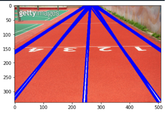
P4. (Hough Line) 다음 그림을 이용하여 Hough Line 을 적용하여 보라.

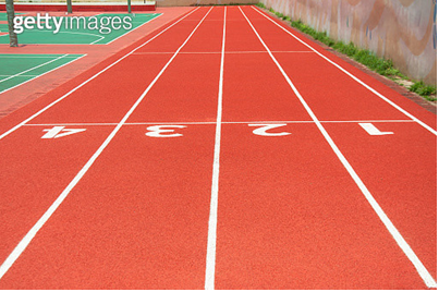
1) 2차원 Gaussian 필터의 파라메터를 조절하면서 Hough 선이 잘 검출되도록 하라.

<코드>

import cv2
import numpy as np
from matplotlib import pyplot as plt
'''
1)     2차원 Gaussian 필터의 파라메터를 조절하면서 Hough 선이 잘 검출 되도록 하라.
'''
img=cv2.imread('p4.png')

def myHough(src,sigma):
    #원본이미지 복사
    orig=src
    img_gray = cv2.cvtColor(src, cv2.COLOR_BGR2GRAY)

    #가우시안 필터링
    img = cv2.GaussianBlur(img_gray,(13,13),sigma)

    #캐니 에지
    img_canny = cv2.Canny(img, 50, 150, apertureSize = 3)

    #패러미터는 이미지, 로 해상도, 세타 해상도, threshold
    lines = cv2.HoughLines(img_canny, 1, np.pi/180, 100)

    #rho, theta로 표현된 직선을 직교좌표계로 변환
    for i, line in enumerate(lines):
        rho,theta = line[0]     # rho and theta
        a = np.cos(theta)       # x sin(theta) + y cos(theta) = rho
        b = np.sin(theta)
        x0 = a*rho              # 수직교점
        y0 = b*rho
        t = 1000
        x1 = int(x0 + t*(-b))
        y1 = int(y0 + t*(a))
        x2 = int(x0 - t*(-b))
        y2 = int(y0 - t*(a))

        #라인 그리기
        cv2.line(orig,(x1,y1),(x2,y2),(255,0,0),3)
    return orig

final = myHough(img, 2)

final = cv2.cvtColor(final, cv2.COLOR_BGR2RGB)
plt.imshow(final)
plt.show()

<결과>

2) 위에서 얻은 라인들중에서 래인들을 위한 조건을 이용하여 레인들에 해당하는 선들만 남겨라. (OpenCV는 theta 가 0 – 180 도로 주어지는 것에 주의 할 것, 따라서 수평라인은 90도.)

<코드>

def myHough(src,sigma):
    #원본이미지 복사
    orig=src
    img_gray = cv2.cvtColor(src, cv2.COLOR_BGR2GRAY)

    #가우시안 필터링
    img = cv2.GaussianBlur(img_gray,(13,13),sigma)

    #캐니 에지
    img_canny = cv2.Canny(img, 50, 150, apertureSize = 3)

    #패러미터는 이미지, 로 해상도, 세타 해상도, threshold
    lines = cv2.HoughLines(img_canny, 1, np.pi/180, 100)

    #rho, theta로 표현된 직선을 직교좌표계로 변환
    for i, line in enumerate(lines):
        rho,theta = line[0]     # rho and theta
      a = np.cos(theta)       # x sin(theta) + y cos(theta) = rho
        b = np.sin(theta)
        x0 = a*rho              # 수직교점
        y0 = b*rho
        t = 1000
        x1 = int(x0 + t*(-b))
        y1 = int(y0 + t*(a))
        x2 = int(x0 - t*(-b))
        y2 = int(y0 - t*(a))

        #라인 그리기
        #함수 수정
        if not(rho > 0 and theta > np.pi/2):
            cv2.line(orig,(x1,y1),(x2,y2),(255,0,0),3)

    return orig

final = myHough(img, 2)

final = cv2.cvtColor(final, cv2.COLOR_BGR2RGB)
plt.imshow(final)
plt.show()

<결과>

3) 다음 이미지에 대하여 위 알고리즘을 적용하여 보라. 어떤 문제가 있는가?

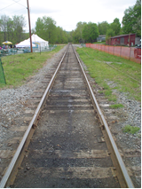
<코드>

img2 = cv2.imread('p4_2.png')

final2 = myHough(img2, 3)

final2 = cv2.cvtColor(final2, cv2.COLOR_BGR2RGB)
plt.imshow(final2)
plt.show()

<결과>

선로의 아래쪽 부분이 잘 검출되지 않았으며 왼쪽의 전신주 또한 같이 검출되었다.

원본 이미지에서 선로와 배경간의 색상차이가 얼마 나지 않아 생긴 문제일 것이다.

P5. [영역분할] 다음 이미지를 보고 등불의 개수를 카운팅하는 프로그램을 작성하려고 한다.

(1) 다음 이미지를 전처리을 수행하고 이진화 및 후 처리하여 영역분할하라.

(2) 위의 영역분할의 결과를 이용하여 찾은 전구의 위치를 표시하고 번호를 매겨서, 개수를 학인 해보라.

*1,2번 동시 수행

<코드>

import cv2
import numpy as np
from matplotlib import pyplot as plt

img = cv2.imread('p5.png')

def region(src):
    #오리지널 영상 저장
    orig= src
    #흑백으로 변경
    src = cv2.cvtColor(src, cv2.COLOR_BGR2GRAY)

    #오츄 알고리즘 사용 이진화
    # + cv2.THRESH_OTSU
    thres, im_bin = cv2.threshold(src, thresh = 230 , maxval = 255, type = cv2.THRESH_BINARY)

    #모폴로지컬 필터 사용
    #erosion 함수, 뒤의 패러미터는 몇번 적용할 것인가
    kernel = np.ones((3,3),np.uint8)
    #하얀색 영역 내에 있는 모든 노이즈 제거.(안 하면 영역이 여러개 나온다)
    im_bin = cv2.morphologyEx(im_bin, cv2.MORPH_CLOSE, kernel)

    erosion = cv2.erode(im_bin,kernel,iterations = 5)
    dilation = cv2.dilate(erosion,kernel,iterations = 5)

    retval, labels, stats, centroids= cv2.connectedComponentsWithStats(dilation)
    print('retval=',retval)

    #인덱스 0은 배경을 의미하기 때문에 1부터 시작
    m=1
    while(m<retval):
        orig = cv2.circle(orig, (int(centroids[m,0]),int(centroids[m,1])) ,20 , (0,0,255), thickness=5)
        m=m+1

    plt.imshow(orig[:,:,::-1])
    plt.axis('off')
    plt.title('counting')
    plt.show()


region(img)

<결과>

P6. [Grabcut] Grab-cut을 이용한 이미지 블렌딩을 수행해본다.

1) 수업에서 사용한 마스크 드로잉 코드들 활용하고 Grabcut 함수를 이용하여 다음 악어를 잘라내라.

<코드 - 드로잉>

img = cv2.imread('p6_1.png') # 입력 영상
mask = np.ones([img.shape[0], img.shape[1]], dtype = 'uint8') * 128 # 패인트 작업 저장

###########################
#드로잉 코드로 마스크 영상 만들기
###########################

key_pressed = False
mouse_pressed = False
color = 0

# 마우스에 특정 이벤트가 밸생하면 호출됨
def mouse_callback(event, x, y, flags, param):

    print('event:', event, 'x:', x, 'y:', y, 'flags:', flags)

    global mouse_pressed, key_pressed, color # 함수 외부에 선언된 변수를 사용하기 위한 선언

    if event == cv2.EVENT_LBUTTONDOWN:
        mouse_pressed = True
        cv2.circle(img, (x, y), 5, (color, color, color), cv2.FILLED)
        cv2.circle(mask, (x, y), 5, color, cv2.FILLED)

    elif event == cv2.EVENT_MOUSEMOVE:
        if mouse_pressed:
            cv2.circle(img, (x, y), 5, (color, color, color), cv2.FILLED)
            cv2.circle(mask, (x, y), 5, color, cv2.FILLED)
    elif event == cv2.EVENT_LBUTTONUP:
        mouse_pressed = False


cv2.namedWindow('image')
cv2.setMouseCallback('image', mouse_callback)

while True:
    cv2.imshow('image', img)

    k = cv2.waitKey(1) # 이 안에서 기다리다가 마우스 이벤트가 발생하면 콜백을 호출하고, 키보드 입력은 반환이 됨.

    if k == ord('c'): # 종료 명령
        cv2.imwrite('mask.png', mask)
        break
    elif k == ord('0'): # 0은 배경 지정
        color = 0 #(0,0,0)
    elif k == ord('1'): # 1은 전경 지정
        color = 255 #(255,255,255)


cv2.destroyAllWindows()

#################################################

<코드 - 검출>

mask = np.zeros(img.shape[:2],np.uint8)
bgdModel = np.zeros((1,65),np.float64) #13X5=65. (GMM -5), weight, mean 3개. (RGB라 3개), 3X3=9개
fgdModel = np.zeros((1,65),np.float64)

rect=(45,95,1050,650)
cv2.grabCut(img,mask,rect,bgdModel,fgdModel,1,cv2.GC_INIT_WITH_RECT)

img1 = img*np.where((mask==2)|(mask==0),0,1).astype('uint8')[:,:, np.newaxis]
#0=확실한 백그라운드 의미, 2=아마도 백그라운드 의미. 즉 조건연산자로 작동. mask가 0 OR 2면 0대입 아니면 1 대입
#np.newaxis? img와 np.where의 곱셈을 위해 차원 캐스팅

mask1 = mask.copy()

newmask = cv2.imread('mask.png',0)
mask[newmask == 0] = 0
mask[newmask == 255] = 1

cv2.grabCut(img,mask,None,bgdModel,fgdModel,1,cv2.GC_INIT_WITH_MASK)
mask2 = np.where((mask==2)|(mask==0),0,1).astype('uint8')
img2 = img*mask2[:,:,np.newaxis]

plt.subplot(2,2,1), plt.imshow(mask, cmap='gray'), plt.title('after mask'), plt.axis('off')
plt.subplot(2,2,2), plt.imshow(img2[:,:,::-1]), plt.title('final'), plt.axis('off')

plt.show()

<결과>

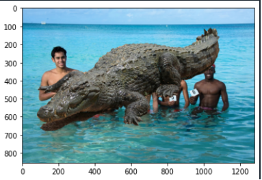
2) 위에서 얻어진 masked image를 크기를 조절하여 다음 영상의 앞부분 위치에 오버라이드 (덮어쓰기)하여 합성하라.

<코드>

'''
2) 위에서 얻어진 masked image를 크기를 조절하여 다음 영상의
앞부분 위치에 오버라이드 (덮어쓰기)하여 합성하라.
'''

img_back = cv2.imread('p6_2.png')
img_croc = cv2.imread('after.png')

#오버라이드. 악어 이미지에서 화소값이 (0,0,0)이 아닌 부분을 background 이미지에 붙여넣기

m=0
n=0

msize,nsize = 787,1199
while(m < msize):
    while(n < nsize):
        b,g,r = img_croc[m][n]
        B,G,R = img_back[m][n]

        if((img_croc[m,n,0]!=0)&(img_croc[m,n,1]!=0)&(img_croc[m,n,2]!=0)):
            img_back[m,n,0]=img_croc[m,n,0]
            img_back[m,n,1]=img_croc[m,n,1]
            img_back[m,n,2]=img_croc[m,n,2]
        n=n+1
    m=m+1
    n=0

plt.imshow(img_back[:,:,::-1])
plt.show()

<결과>

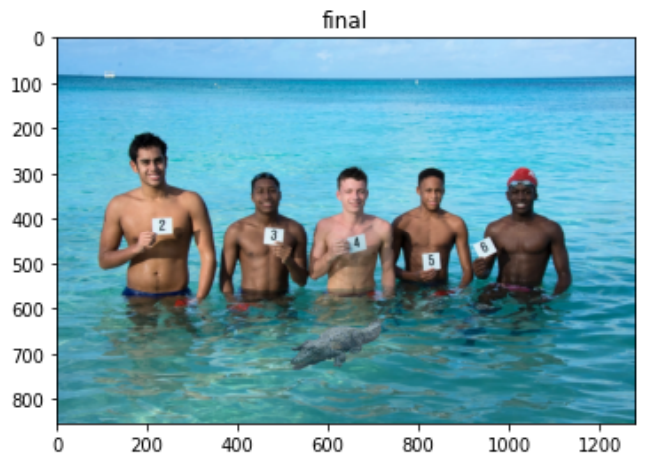
3) 좀더 자연스러운 결과를 보이기 위하여 alpha blending 기법을 이용하라. 즉, 악어의 바운더리 영역에 점차 alpha 값을 조절하라. (cv2.distanceTransform 을 활용할 수 있다.)

<코드>

img_back = cv2.imread('p6_2.png')
img_croc = cv2.imread('after.png')

#test
plt.imshow(img_croc)
plt.title('original')
plt.show()

#사이즈 조절
img_croc = cv2.resize(img_croc,dsize=(0,0),fx=0.2,fy=0.2,interpolation=cv2.INTER_LINEAR)

plt.imshow(img_croc)
plt.title('original_resize')
plt.show()

#오버라이드. 악어 이미지에서 화소값이 (0,0,0)이 아닌 부분을 background 이미지에 붙여넣기

m=0
n=0

dy=600
dx=500

msize,nsize,tmp = np.shape(img_croc)
alp=0.7
while(m < msize):
    while(n < nsize):
        b,g,r = img_croc[m][n]
        B,G,R = img_back[m+dy][n+dx]

        if((img_croc[m,n,0]!=0)&(img_croc[m,n,1]!=0)&(img_croc[m,n,2]!=0)):

            img_back[m+dy,n+dx,0]=alp*img_croc[m,n,0] + (1-alp)*img_back[m,n,0]
            img_back[m+dy,n+dx,1]=alp*img_croc[m,n,1] + (1-alp)*img_back[m,n,1]
            img_back[m+dy,n+dx,2]=alp*img_croc[m,n,2] + (1-alp)*img_back[m,n,2]
        n=n+1
    m=m+1
    n=0

plt.imshow(img_back[:,:,::-1])
plt.title('final')
plt.show()

<결과>

참고 자료

컴퓨터 비전(Computer Vision)

기본 개념부터 최신 모바일 응용 예까지

저자

오일석
출판

한빛아카데미
출간

2014.07.30.

저작자표시

'프로그래밍 > 영상처리공학' 카테고리의 다른 글

[영상처리공학/OpenCV with python]연주 영상 인식 피아노 (0)	2022.12.19
[HW 2]히스토그램, 이진 영상, Morphology 필터 & 기하변환 (0)	2022.12.18
[HW 1]영상처리 기본, Python & OpenCV (0)	2022.12.18

현재글[HW 3]에지 검출과 영역 분할

공부 기록

Today :
Yesterday :

미래로